The garbage man is a complicated piece of equipment that can be challenging to tune. Certainly, the G1 collector alone has more than 20 tuning flags. Not remarkably, lots of designers fear touching the GC. If you do not offer the GC simply a bit of care, your entire application may be running suboptimal. So, what if we inform you that tuning the GC does not need to be tough? In reality, simply by following an easy dish, your GC and your entire application might currently get an efficiency increase.
This post demonstrates how we got 2 production applications to carry out much better by following basic tuning actions. In what follows, we reveal you how we got a 2 times much better throughput for a streaming application. We likewise reveal an example of a misconfigured high-load, low-latency REST service with a generously big stack. By taking some basic actions, we decreased the stack size more than ten-fold without jeopardizing latency. Prior to we do so, we’ll initially discuss the dish we followed that enlivened our applications’ efficiency.
A basic dish for GC tuning
Let’s start with the active ingredients of our dish:
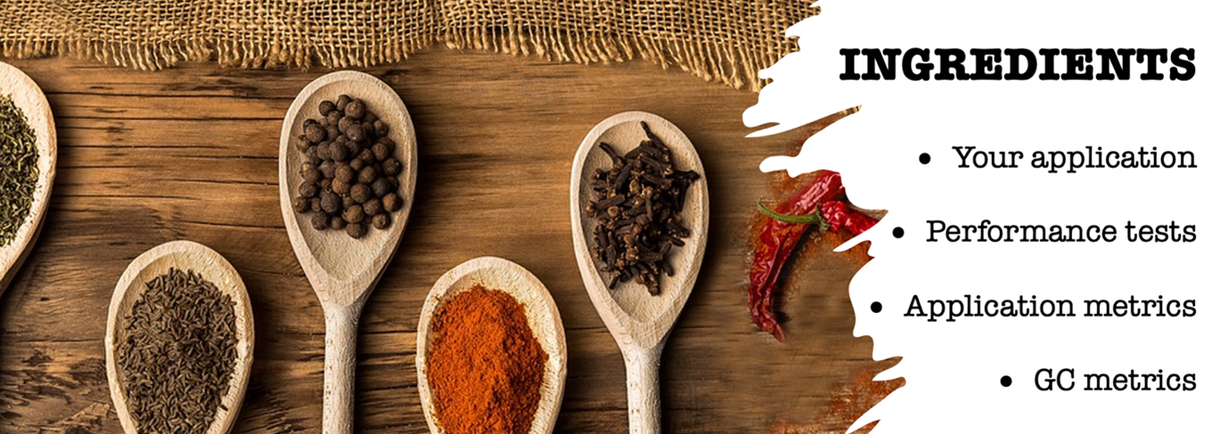
Besides your application that requires spicing, you desire some method to create a production-like load on a test environment – unless feeling brave enough to make performance-impacting modifications in your production environment.
To evaluate how excellent your app does, you require some metrics on its essential efficiency indications. Which metrics depend upon the particular objectives of your application. For instance, latency for a service and throughput for a streaming application. Besides those metrics, you likewise desire details about just how much memory your app takes in. We utilize Micrometer to catch our metrics, Prometheus to extract them, and Grafana to envision them.
With your app metrics, your essential efficiency indications are covered, however in the end, it is the GC we like to enliven. Unless having an interest in hardcore GC tuning, these are the 3 essential efficiency indications to identify how excellent of a task your GC is doing:
- Latency – the length of time does a single trash gathering occasion pause your application.
- Throughput – just how much time does your application invest in trash gathering, and just how much time can it invest in doing application work.
- Footprint – the CPU and memory utilized by the GC to perform its task
This last active ingredient, the GC metrics, may be a bit harder to discover. Micrometer exposes them. (See for instance this post for an introduction of metrics.) Additionally, you might acquire them from your application’s GC logs. (You can describe this short article to find out how to acquire and examine them.)
Now we have all the active ingredients we require, it’s time for the dish:
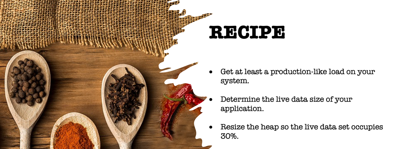
Let’s get cooking. Fire up your efficiency tests and keep them running for a duration to heat up your application. At this moment it is excellent to jot down things like reaction times, optimum demands per second. In this manner, you can compare various runs with various settings later on.
Next, you identify your app’s live information size (LDS). The LDS is the size of all the items staying after the GC gathers all unreferenced items. To put it simply, the LDS is the memory of the items your app still utilizes. Without entering into excessive information, you should:
- Trigger a complete trash gather, which requires the GC to gather all unused items on the stack. You can set off one from a profiler such as VisualVM or JDK Objective Control
- Check out the utilized stack size after the complete gather. Under typical situations you must have the ability to quickly acknowledge the complete gather by the big drop in memory. This is the live information size.
The last action is to recalculate your application’s stack. In many cases, your LDS must inhabit around 30% of the stack ( Java Efficiency by Scott Oaks). It is excellent practice to set your very little stack (Xms) equivalent to your optimum stack (Xmx). This avoids the GC from doing pricey complete gathers on every resize of the stack. So, in a formula: Xmx = Xms = max( LDS)/ 0.3
Enlivening a streaming application
Envision you have an application that processes messages that are released on a line. The application runs in the Google cloud and utilizes horizontal pod autoscaling to instantly scale the variety of application nodes to match the line’s work. Whatever appears to run fine for months currently, however does it?
The Google cloud utilizes a pay-per-use design, so including additional application nodes to improve your application’s efficiency comes at a cost. So, we chose to try our dish on this application to see if there’s anything to get here. There definitely was, so continue reading.
Prior To
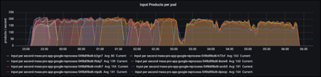
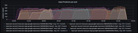
To develop a standard, we ran an efficiency test to get insights into the application’s essential efficiency metrics. We likewise downloaded the application’s GC logs to get more information about how the GC acts. The listed below Grafana control panel demonstrates how lots of components (items) each application node procedures per second: max 200 in this case.
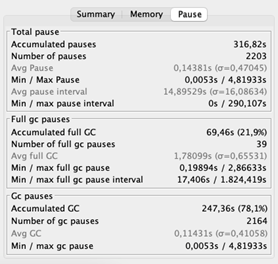
These are the volumes we’re utilized to, so all excellent. Nevertheless, while examining the GC logs, we discovered something that stunned us.

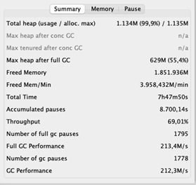
The typical time out time is 2,43 seconds. Remember that throughout stops briefly, the application is unresponsive. Long hold-ups do not require to be a problem for a streaming application due to the fact that it does not need to react to customers’ demands. The stunning part is its throughput of 69%, which indicates that the application invests 31% of its time erasing memory. That is 31% not being invested in domain reasoning. Preferably, the throughput must be at least 95%.
Figuring out the live information size
Let us see if we can make this much better. We identify the LDS by activating a complete trash gather while the application is under load. Our application was carrying out so bad that it currently carried out complete gathers– this normally shows that the GC remains in difficulty. On the intense side, we do not need to set off a complete gather by hand to find out the LDS.
We distilled that limit stack size after a complete GC is roughly 630MB. Using our general rule yields a load of 630/ 0.3 = 2100MB. That is practically two times the size of our existing stack of 1135MB!
After
Curious about what this would do to our application, we increased the stack to 2100MB and fired up our efficiency tests once again. The outcomes thrilled us.

After increasing the stack, the typical GC stops briefly reduced a lot. Likewise, the GC’s throughput enhanced considerably– 99% of the time the application is doing what it is planned to do. And the throughput of the application, you ask? Remember that previously, the application processed 200 components per second at the majority of. Now it peaks at 400 per 2nd!
Enlivening a high-load, low-latency REST service
Test concern. You have a low-latency, high-load service working on 42 virtual devices, each having 2 CPU cores. Someday, you move your application nodes to 5 monsters of physical servers, each having 32 CPU cores. Considered that each virtual device had a load of 2GB, what size should it be for each physical server?
So, you should divide 42 * 2 = 84GB of overall memory over 5 devices. That comes down to 84/ 5 = 16.8 GB per device. To take no possibilities, you round this number as much as 25GB. Sounds possible, best? Well, the proper response seems less than 2GB, since that’s the number we managed determining the stack size based upon the LDS. Can’t think it? No concerns, we could not think it either. For that reason, we chose to run an experiment.
Experiment setup
We have 5 application nodes, so we can run our explore 5 differently-sized stacks. We offer node one 2GB, node 2 4GB, node 3 8GB, node 4 12GB, and node 5 25GB. (Yes, we are not brave enough to run our application with a load under 2GB.)
As a next action, we fire up our efficiency tests producing a steady, production-like load of a complicated 56K demands per second. Throughout the entire run of this experiment, we determine the variety of demands each node gets to guarantee that the load is similarly well balanced. What is more, we determine this service’s essential efficiency indication– latency.
Since we got tired of downloading the GC logs after each test, we bought Grafana control panels to reveal us the GC’s time out times, throughput, and stack size after a trash gather. In this manner we can quickly examine the GC’s health.
Outcomes
This blog site has to do with GC tuning, so let’s begin with that. The following figure reveals the GC’s time out times and throughput. Remember that time out times suggest the length of time the GC freezes the application while purging memory. Throughput then defines the portion of time the application is not stopped briefly by the GC.
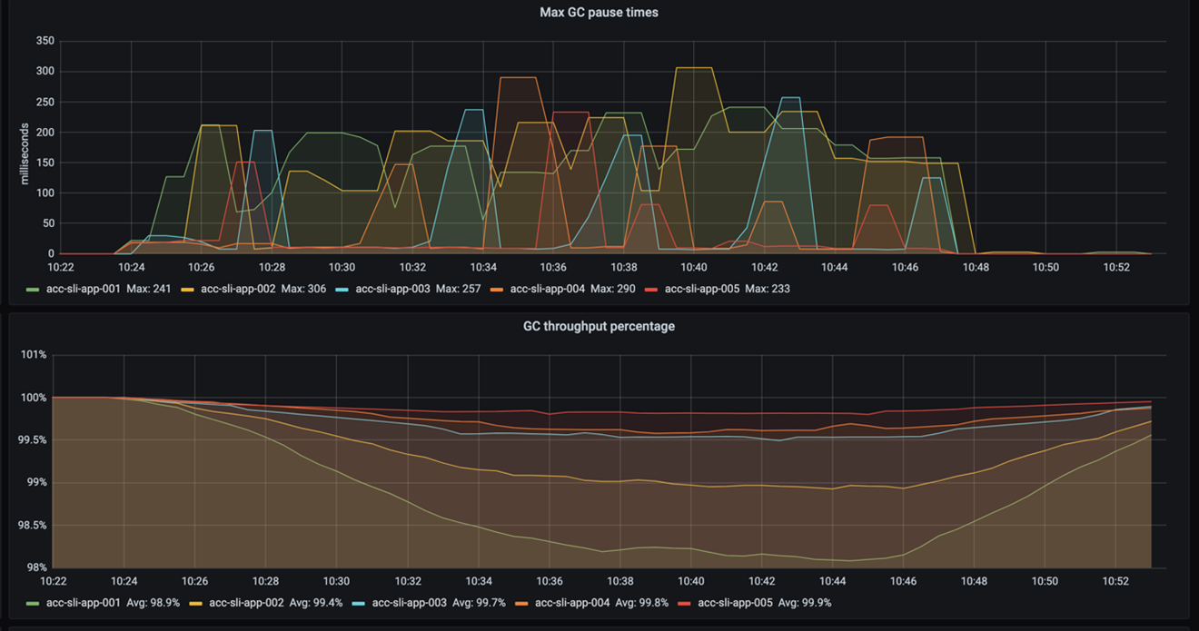
As you can see, the time out frequency and time out times do not vary much. The throughput reveals it finest: the smaller sized the stack, the more the GC stops briefly. It likewise reveals that even with a 2GB stack the throughput is still okay– it does not drop under 98%. (Remember that a throughput greater than 95% is thought about excellent.)
So, increasing a 2GB stack by 23GB increases the throughput by practically 2%. That makes us question, how considerable is that for the general application’s efficiency? For the response, we require to take a look at the application’s latency.
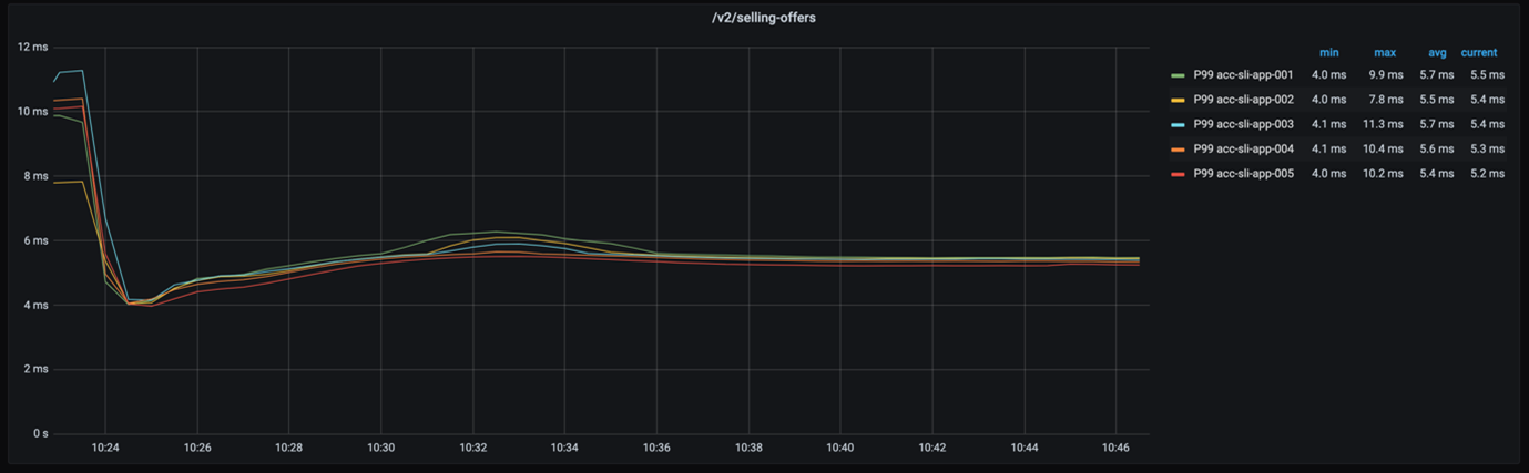
If we take a look at the 99-percentile latency of each node– as displayed in the listed below chart– we see that the reaction times are truly close.
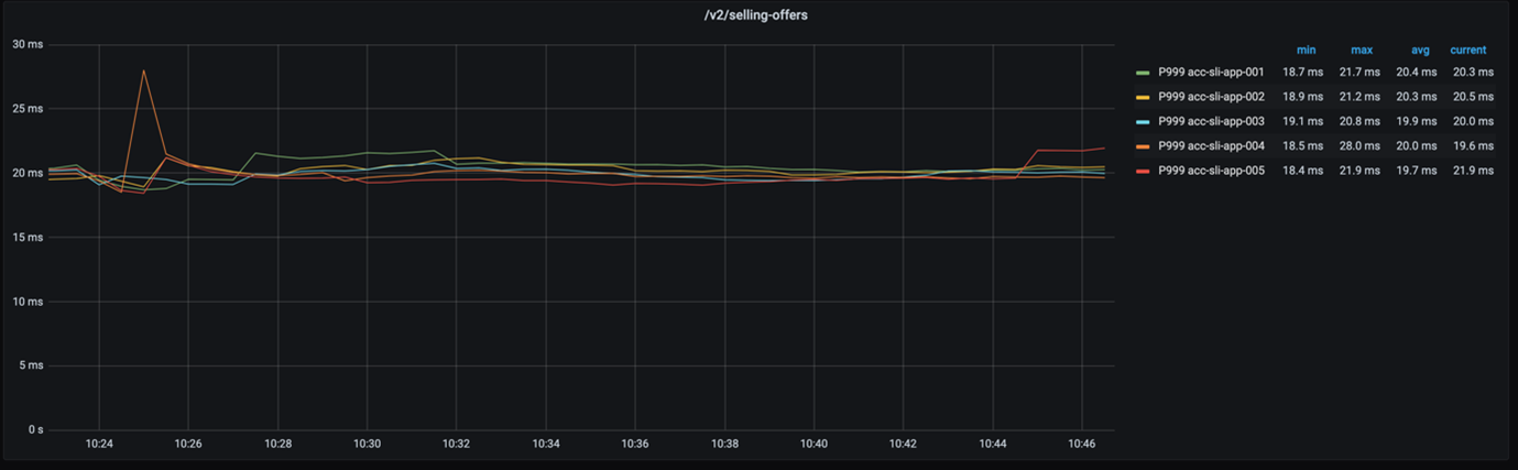
Even if we think about the 999-percentile, the reaction times of each node are still not really far apart, as the following chart programs.
How does the drop of practically 2% in GC throughput impact our application’s general efficiency? Very little. Which is fantastic due to the fact that it indicates 2 things. Initially, the basic dish for GC tuning worked once again. Second, we simply conserved a tremendous 115GB of memory!
Conclusion
We discussed an easy dish of GC tuning that served 2 applications. By increasing the stack, we got 2 times much better throughput for a streaming application. We decreased the memory footprint of a REST service more than ten-fold without jeopardizing its latency. All of that we achieved by following these actions:
⢠Run the application under load.
⢠Identify the live information size (the size of the items your application still utilizes).
⢠Size the stack such that the LDS takes 30% of the overall stack size.
Ideally, we encouraged you that GC tuning does not require to be intimidating. So, bring your own active ingredients and begin cooking. We hope the outcome will be as spicy as ours.
Credits
Lots of thanks to Alexander Bolhuis, Ramin Gomari, Tomas Sirio and Deny Rubinskyi for assisting us run the experiments. We could not have actually composed this post without you men.